In this blog post, I want to explain a way in which I like to motivate Lie groupoids via the theorem on the existence and uniqueness of solutions to ordinary differential equations. The basic idea is that in trying to do away with the choices – the initial time and the initial conditions – we’re naturally led to consider a ‘universal fundamental solution’. This is a matrix function depending on two parameters, the initial and final times, and it must satisfy a homomorphism-type condition. In order to axiomatize this condition, we are automatically led to the definition of a Lie groupoid. Once this has been absorbed, we can then rephrase the existence and uniqueness theorem as a correspondence between ODEs and representations of the pair groupoid of the real line. This is a special case of Lie’s second theorem for Lie groupoids.
1. Ordinary differential equations
To begin, let’s consider first order linear homogeneous ordinary differential equations. These are differential equations of the following form

where  is the independent variable,
  is a given known function, and
  is an unknown function. More generally, we could consider systems of the following form

Such a system can be compactly expressed in terms of matrices as follows
 (1)
(1)
where  is a column vector consisting of
  unknown functions, and
  is the
  matrix of functions

For simplicity, I’m going to assume that the functions  are smooth, i.e. infinitely differentiable:
  . A solution to such a differential equation is a function
  which satisfies equation (1). The following fundamental theorem guarantees the existence and uniqueness of solutions.
Theorem 1. Given the choice of an initial condition  and an initial time
  , there is a unique solution
  of equation (1) which satisfies

Solutions to equation (1) are closed under linear combinations and therefore form a vector space. This is because equation (1) is linear. As a result, it suffices to find solutions with initial conditions given by a basis of  , such as

and where  has a single non-zero entry in the
  row. Putting these solutions together as the columns of an matrix gives a fundamental solution. This is a function
  , valued in matrices
  , which solves the matrix equation

subject to the initial condition  . The solution with initial condition
  is then recovered as
  .
.
One of the reasons to introduce the fundamental solution to equation (1) is to remove the dependence on initial conditions. However, there still remains the choice of ‘initial time’  . Getting rid of this gives rise to the parallel transport of the differential equation.
Definition 2. The parallel transport of equation (1) is the function

defined by letting  be the matrix solution to equation (1) satisfying the initial condition

I like to think of the parallel transport as the universal fundamental solution since it contains within it all fundamental solutions and is uniquely determined by the differential equation (1). The terminology indicates that we should also think of  as a linear map which transports vectors from a copy of lying above to a copy of lying above
  .
.
Corollary 3 (Algebraic properties of parallel transport). The parallel transport  of equation (1) satisfies the following properties:
 for all
  ,
, for all
  ,
, (i.e. is invertible) for all
  .
.
Proof. Property 1 follows because of the initial condition in the definition of the parallel transport, and property 3 follows from 1 and 2. To prove 2, let  and
and  for fixed values of
  . Then
  and
and  both satisfy equation (1). Furthermore,
  by 1, and
  . Therefore
  by uniqueness of the solutions.
2. Lie groupoids
The upshot of Corollary 3 is that given the differential equation (1), we solve it to produce the parallel transport map

which satisfies

for all  . This equation should call to mind the concept of a group homomorphism. Indeed, if we define
  , then the above equation reads

However,  is not a group: the product
  should only be defined if
  . In fact, is a groupoid over
  , which is known as the pair groupoid
  .
.
I now want to briefly pause this discussion to give you the general definition of a groupoid. A groupoid consists of two sets: a set of ‘arrows’  and a set of ‘objects’
  . We view the elements
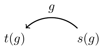
  literally as arrows connecting points of the base :
In this way, every arrow  has a source
  and a target
  , and this defines two maps

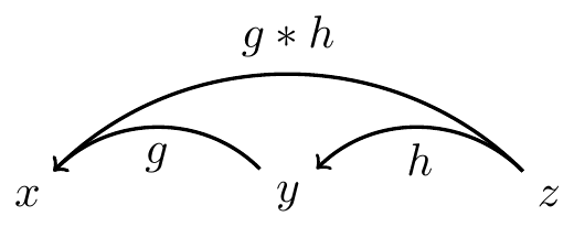
In addition, the set of arrows is equipped with a partial multiplication which allows us to compose two arrows which match ‘tip-to-tail’. To make this precise, we define the set of composable arrows as follows

The multiplication is then a map

and it should be pictured in the following way
As is clear from the diagram, the multiplication map must satisfy

It should also satisfy the usual associativity condition  , when this is defined. In addition, for each object
  , there is a distinguished arrow
  , with
  , which acts as an identity for the multiplication. This defines a map

Finally, every arrow should be invertible, in the sense that there is an inverse  which satisfies

I will generally denote a groupoid by  , or more simply by when the base is understood.
Given any set , the pair groupoid  is a groupoid with set of objects and set of morphisms
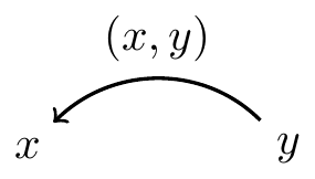
  . We view pairs
  as arrows connecting points of as follows:
so that  and
and  . Since there is a unique arrow connecting any two points, the multiplication is then forced to be given by

and the identity above  is given by
  .
.
There are myriad examples of groupoids and I’ll mention a few more. Any group  defines a groupoid
  in which the set of objects consists of a single point. Therefore, groupoids generalize groups by allowing more than one identity element. At the other extreme, any set defines a groupoid
  which contains only identity arrows.
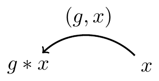
For a more interesting example, given a set with a left action of a group , we may form the action groupoid  , which has set of objects and set of arrows
  . A pair
  defines an arrow in the following way
and the multiplication is inherited from the product in .
As a final example, given a topological space  , the fundamental groupoid
  is the groupoid over whose set of morphisms consists of continuous paths
 ![\gamma: [0,1] \to M](https://s0.wp.com/latex.php?latex=%5Cgamma%3A+%5B0%2C1%5D+%5Cto+M&bg=%23ffffff&fg=000000&s=0&c=20201002) , considered up to homotopies with fixed endpoints. The source and target maps are respectively given by the endpoints
, considered up to homotopies with fixed endpoints. The source and target maps are respectively given by the endpoints  and
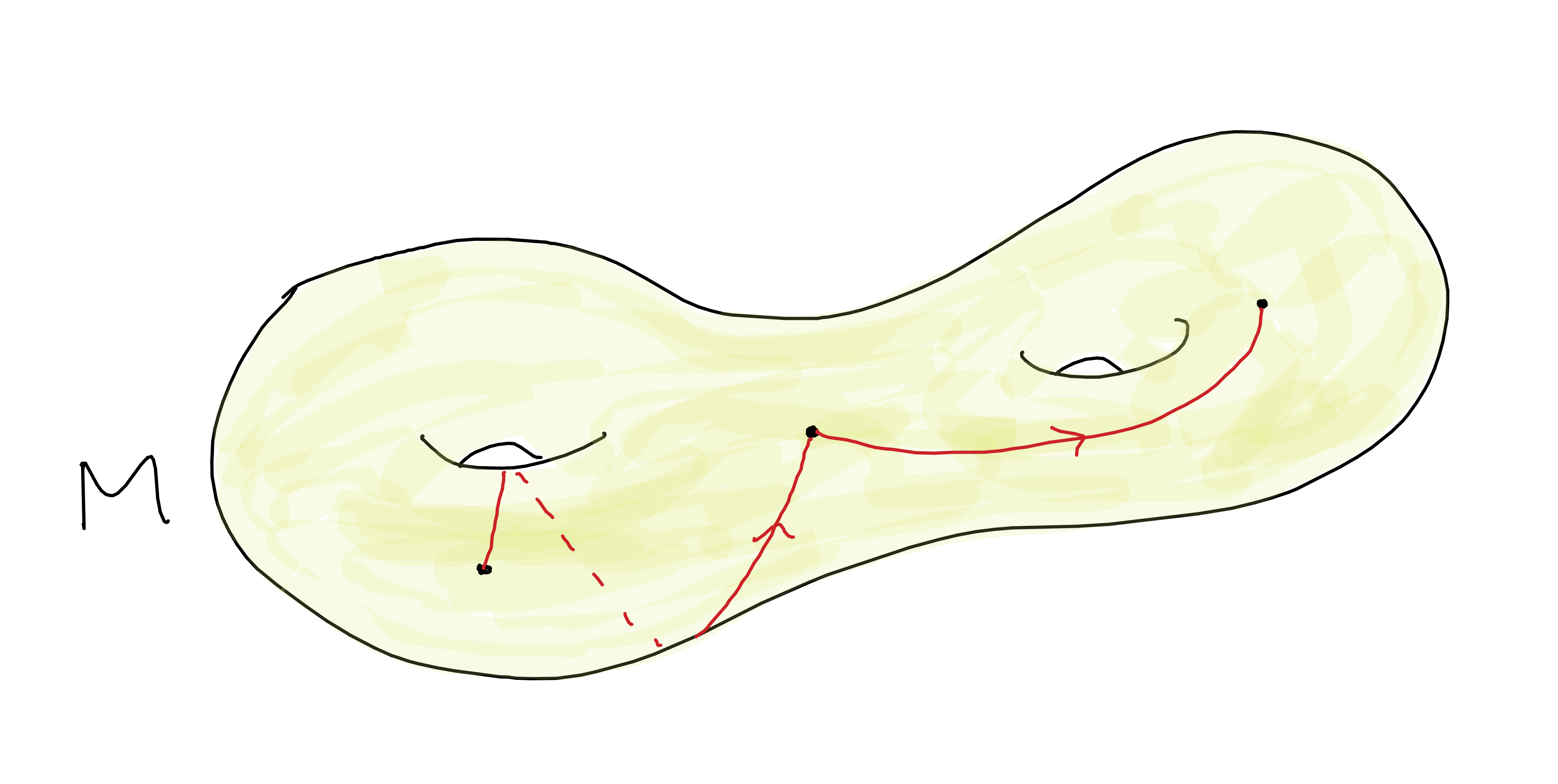
and  , and the multiplication is given by concatenation of paths. A picture of two morphisms being composed is given in the following picture.
The example from the beginning of this section is actually an instance of several of the above examples. Indeed, consider the addition action of on itself. In the action groupoid  there is a unique arrow between any two points and as a result
  . Furthermore,
  . This is because there is a unique homotopy class of path in connecting any two points.
Returning to Corollary 3 we now see that the parallel transport of equation (1) defines a homomorphism between two groupoids:

In fact, something stronger is true: both and  are smooth manifolds, and
  is a smooth map. In other words, is a Lie groupoid homomorphism.
More generally, a Lie groupoid is a groupoid in which the set of objects and the set of morphisms are both smooth manifolds, such that the structure maps  are smooth, and such that
  and
and  are surjective submersions. This last condition is required in order to ensure that the space of composable arrows
  is a smooth manifold. All of the examples of groupoids I gave above are actually examples of Lie groupoids (at leasts when the sets involved are smooth manifolds). I’ll leave the definition of a (Lie) groupoid homomorphism for you to figure out.
Finally, I can now state a reformulation of the existence and uniqueness theorem for ODEs in the language of Lie groupoids.
Theorem 4. There is a one-to-one correspondence between linear ODEs of the form (1) and representations of the pair groupoid :

where is the parallel transport of the ODE  .
.
Proof. One direction of this correspondence, sending an ODE specified by  to the parallel transport , is covered by Corollary 3. In the opposite direction, given a homomorphism , the ODE is defined as follows:
 (2)
(2)
We will show that these two maps are inverse to each other. First, it follows by definition that when is the parallel transport of the ODE specified by , then equation (2) recovers . In the other direction, suppose that is a homomorphism and that is defined by equation (2). We must show that is the parallel transport of this ODE. Using the homomorphism property, we verify

Remark 5. Theorem 4 is a special case of Lie’s second theorem for Lie groupoids (here, and here). This is a bijection between Lie groupoid homomorphisms and Lie algebroid homomorphisms under certain connectivity conditions on the groupoids. Another special case of this result is the classical version of Lie’s second theorem which gives a bijection between Lie algebra and Lie group homomorphisms.
Remark 6. One of the upshots of the discussion in this section is that the parallel transport, which is the universal fundamental solution to the ODE given by equation (1), is naturally defined on the pair groupoid . This result continues to hold in the holomorphic category and can be extended to the case of differential equations with singularities. However, in the presence of singularities, the fundamental solution can be singular and multi-valued, so that the parallel transport is not well-defined on the pair groupoid  . Instead, the parallel transport is well-defined and holomorphic on another holomorphic Lie groupoid
  whose structure is specifically adapted to the singularities. This perspective is the basis of these two papers: paper1, paper2.