In my last post, I told you how to encode the zero locus of a polynomial function  in terms of an
  -algebra structure on
 ![L = V[-1] \oplus E[-2]](https://s0.wp.com/latex.php?latex=L+%3D+V%5B-1%5D+%5Coplus+E%5B-2%5D+&bg=%23ffffff&fg=000000&s=0&c=20201002) , where
, where  lies in degree
  and
and  lies in degree
  . Namely, we simply defined the
  ary bracket on
  to be the
  Taylor coefficient of
  This gave us one of the simplest examples of a derived manifold: the derived vanishing locus of
  It also illustrated a simple ‘principle’ of derived algebraic geometry: if the equations defining a space are not independent, then don’t impose them. Instead treat the equations as geometric spaces in their own right. This is useful in part because it allows us to avoid dealing directly with the space defined by the equations, which can often be quite pathological.
In this post, I want to discuss the other side of the story: quotients. What if we are trying to define a space by imposing an equivalence relation that fails to be independent in some way? Again the result can be quite pathological and the solution to this problem is, once again, to do nothing: just don’t take the quotient and treat the equivalence relation as a geometric space in its own right. This will lead us to Lie groupoids and then to stacks, which are Lie groupoids up to Morita equivalence. But what I’m really aiming towards is the infinitesimal counterpart to a Lie groupoid, which is called a Lie algebroid. After reviewing the definition I will explain that, by taking the Taylor coefficients of the structure maps, a Lie algebroid can locally be encoded by an -algebra, this time concentrated in degrees  and . This -algebra, considered up to quasi-isomorphisms, encodes the formal quotient stack associated to the Lie algebroid. This post will be a little longer and a bit less concrete than the last one, but I still hope that it will help demystify both stacks and -algebras.
What’s the matter with quotients?
Let’s start with one of the simplest cases of quotients. I have a Lie group  that acts on a manifold
  and I want to take the quotient space
  , defined as the space of orbits, where two points
  are identified if there is an element of the group,
  , sending one to the other:
  . I’d like to know when the resulting space is a manifold. Having taken a differential topology class, I know of a sufficient condition: the action must be free and proper. Instead of recalling what this means, let me just recall a nice example: the additive action of the integers
  on the real numbers
  , whose quotient is a circle:
  .
.
This can be taken as our prototypical example of a free and proper action. If we drop either of these conditions, then the quotient might not be a nice smooth manifold anymore.
For example, we could consider the rotation action of the cyclic group  on the two-dimensional plane
  . This action is proper and almost everywhere free. But it has a non-trivial stabilizer at the origin given by the full cyclic group. The result is that when we take the quotient, we get a cone, which has a singularity at the vertex. Here’s a picture for the cyclic group of order
  :
:
In fact, things can go wrong in much more serious ways, even when we have a free group action. A good example of this is the irrational torus. I’m going to build up to this.
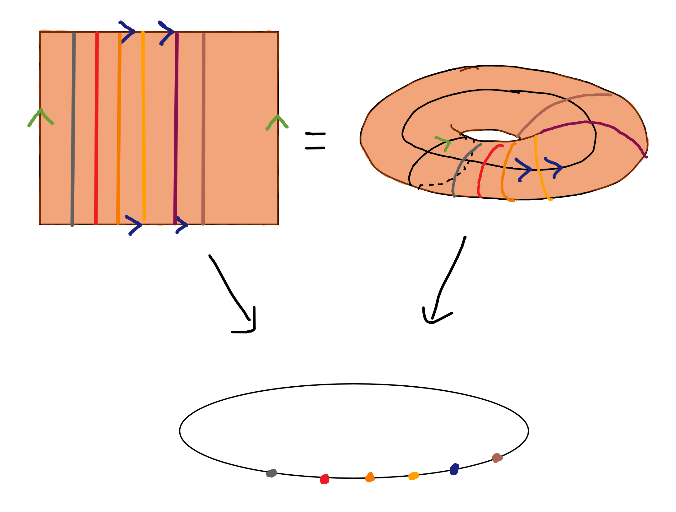
We start with a torus  , which we think of as a square
 ![[0,1]^2](https://s0.wp.com/latex.php?latex=%5B0%2C1%5D%5E2+&bg=%23ffffff&fg=000000&s=0&c=20201002) with opposite sides identified, as follows:
with opposite sides identified, as follows:
Now choose a direction  and consider the action of the real numbers on the torus given by translation in the direction
  . For example, take
  , the vertical direction. Then the orbits of the action are ‘vertical’ circles and the quotient is a circle (note here that we have a nice smooth quotient, even though the action evidently isn’t free).
Or take the direction  . The orbits are now circles that wind once in one direction and twice in the other. The quotient is still a circle.
Now for the irrational torus. For this, take a direction vector with an irrational slope, such as  . In this case, the orbits are no longer loops. Because the slope is irrational, the path will wind around forever, without ever overlapping, but gradually filling up a dense subset of the torus. It’s quite difficult to draw this, but here’s my best attempt. This doesn’t show the full orbit, but maybe something like the orbit for some large interval
 ![[0,100] \subset \mathbb{R}.](https://s0.wp.com/latex.php?latex=%5B0%2C100%5D+%5Csubset+%5Cmathbb%7BR%7D.+&bg=%23ffffff&fg=000000&s=0&c=20201002)
The quotient space  is the irrational torus. In this case, the action of is free but not proper, and the space
  is quite nasty. For example, it is highly non-Hausdorff: because each orbit is dense in the torus, any two orbits get arbitrarily close to each other and cannot be separated.
Lie groupoids
Okay, I got a bit carried away drawing all those pictures, but I hope I’ve convinced you, in case you didn’t already know it, that quotients can be quite nasty in general. As I hinted above, one way to deal with this is simply to refrain from taking the quotient: we deal with the group action as a geometric space in its own right. This brings us to the notion of Lie groupoids. For those who like short and slick definitions: a groupoid is a category where all arrows are invertible and a Lie groupoid is a groupoid internal to the category of smooth manifolds.
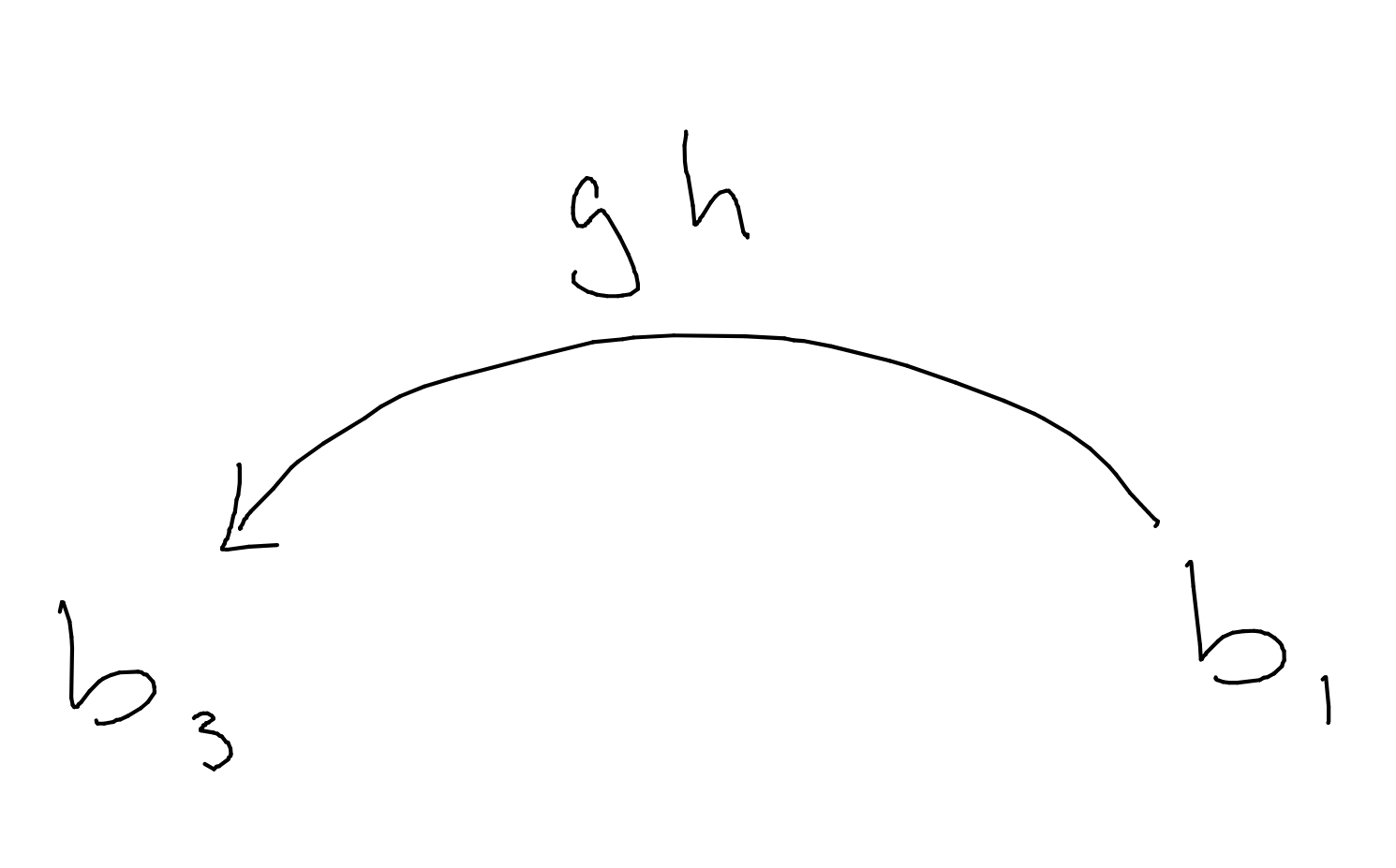
Here’s a slightly more casual definition. A Lie groupoid has two spaces: a space of objects  and a space of arrows
  . We think of points of literally as arrows, or morphisms, connecting two points of the base, like this:
In this picture,  is an arrow going from
  , its source, to
  , its target. This gives us two maps
  . Furthermore, given two arrows
  whose endpoints matchup like this:
then we can compose them to get a new arrow:
This defines a partial multiplication map.

On the left-hand side we have the space of ‘composable arrows’, defined as a fibre product.
In addition, above every point  there is a unit arrow
  which acts as the identity for multiplication. This defines an embedding
  , which is called the identity bisection. Finally, there is a map
  sending every arrow to its inverse.
Note that Lie groups give examples of Lie groupoids. In this case, the space of objects is just a single point. Smooth manifolds also provide examples. Namely, if is a smooth manifold, then we obtain a Lie groupoid by taking  , with the source and target maps given by the identity. In this case, we only have identity arrows, two of which can compose only when they are equal. We conclude from these two examples that Lie groupoids provide a common generalization of both Lie groups and smooth manifolds.
More importantly for our discussion, we also get examples coming from groups acting on manifolds. These are called action groupoids. Let be a Lie group acting on a manifold . Then we take  and
and  . The source map is given by the projection onto :

the target map is given by the action:

and the composition is given by the group multiplication:
 .
.
By the way, people often denote this groupoid as follows: 
It’s worth observing that the action groupoid completely encodes the group action. In particular, the orbits of the action as well as the quotient, which is the space of orbits, can both be determined from the action groupoid. In fact, they are special cases of constructions that make sense for arbitrary Lie groupoids. Indeed, the orbit of a point in the base of a groupoid is defined to be the submanifold of all points which can be connected to  by an arrow:
 .
.
Taking the space of orbits then defines the quotient space of a groupoid
 .
.
Just as in the case of group actions, this is always defined as a topological space, but it may or may not define a smooth manifold.
Crucially though, a groupoid remembers strictly more information than this quotient: it remembers all the ways in which two points of are equivalent to each other. In particular, it remembers all the ways in which a point is related to itself. This set of arrows forms a group which is called the isotropy group of 

In the case of an action groupoid  the isotropy groups are just the stabilizer subgroups of , which measure the failure of the action being free.
Let’s look at the other two examples of Lie groupoids we’ve seen so far. For a Lie group, the base, as well as the quotient space, consists of a single point. On the other hand, the isotropy group is the entire group. For the example coming from a manifold the situation is reversed: the isotropy groups are all trivial, whereas orbits are one-point sets and the quotient space is the manifold .
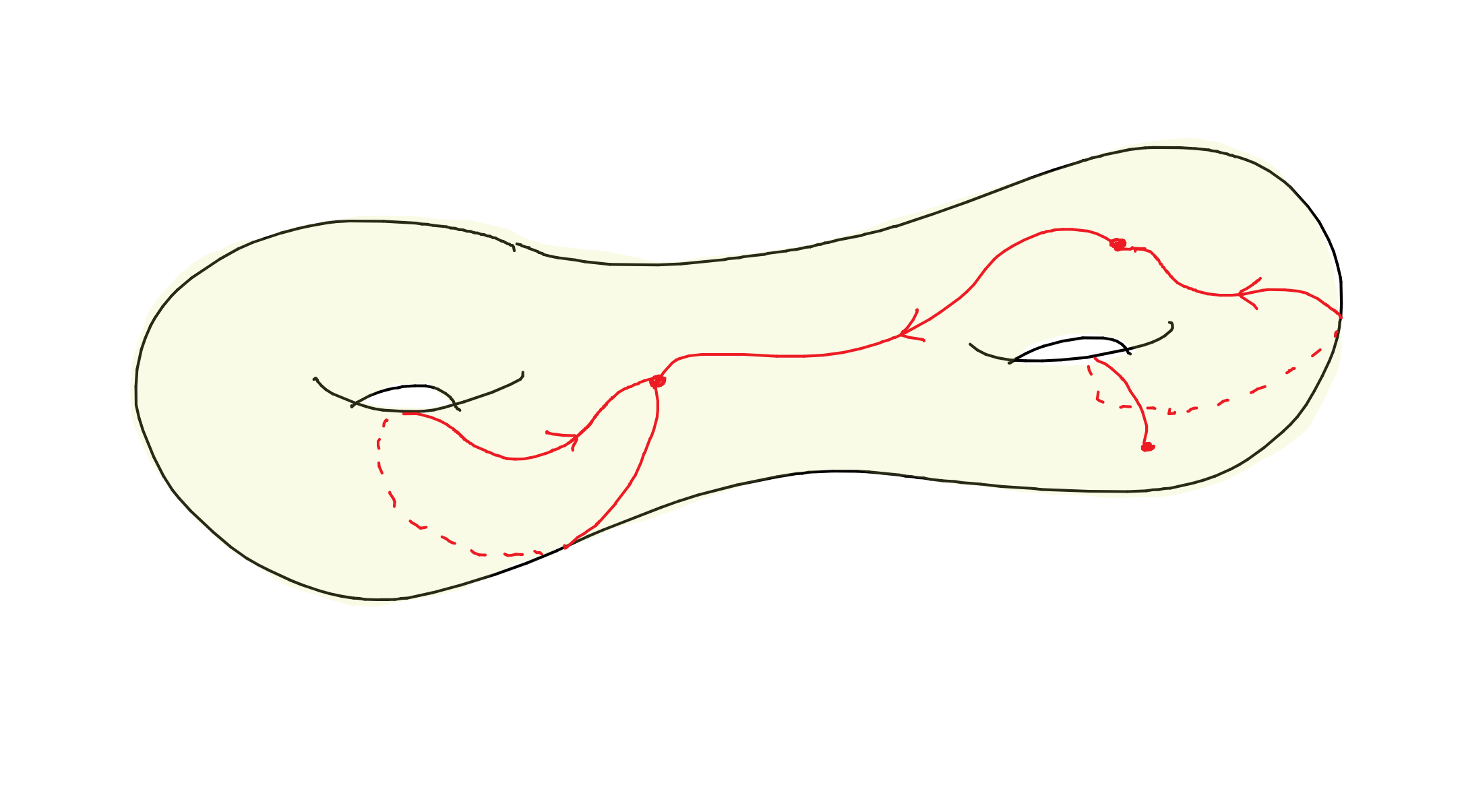
Let’s introduce one more example. Given a manifold , its fundamental groupoid, denoted  , is a groupoid with base and whose space of arrows is the set of homotopy classes of paths in with fixed endpoints:
The source and target of a path are given by the two endpoints and the multiplication is given by path concatenation. In this case, the orbits are the connected components of , so that the quotient space is the set of connected components  . The isotropy group at a point
  is the fundamental group
  .
.
Morita equivalence
We’ve seen that whenever we have a group acting on a manifold , we can define the action groupoid . This is supposed to be some sort of geometric object that replaces the quotient space (which may fail to be smooth). The key to doing this is to remember all the ways in which two points of get identified.
But now we come to a slight problem: the action groupoid remembers too much. To see this, let’s go back to our original example of acting on by translation. On the one hand, this defines an action groupoid  . But on the other hand, the quotient is a well-defined smooth manifold, which may also be viewed as a Lie groupoid. These two groupoids are clearly not the same, even though in some sense they should both represent the same space. We need some way of identifying them.
In fact, there is a well-defined groupoid homomorphism going in one direction

It simply sends an arrow  to the identity arrow above the equivalence class of
  in
in  . This map is particularly nice: it induces a homeomorphism between the quotient spaces as well as isomorphisms between the isotropy groups (which are all trivial)! Hence, even though the map
  does not have an inverse, in some sense it wants to be an equivalence. This is an example of Morita equivalence.
More generally, a Morita equivalence is a kind of identification between two Lie groupoids that, in some sense, want to represent the same space. In order to be more precise, let’s recall that a Lie groupoid is, in particular, a kind of category internal to smooth manifolds. Therefore, a homomorphism between Lie groupoids  can be defined to be a smooth functor. A Morita equivalence is then defined to be a smooth functor that is both essentially surjective and fully faithful. Note that since we are working internally to the category of smooth manifolds, these two terms need to be properly interpreted. I’m not going to do that here. Instead, I’m just going to point out a few consequences of this definition and leave this reference for you to check out (in particular, Section 4).
First, it is generally true that a Morita equivalence induces a homeomorphism between the quotient spaces and an isomorphism between corresponding isotropy groups. In fact, these two properties are almost enough to fully characterize Morita equivalence, but we need a bit more: a functor  also needs to induce an isomorphism between the so-called ‘normal representations’ (see Section 4.3 of the above reference).
Second, if is a Lie group acting freely and properly on a manifold , so that the quotient is a smooth manifold, then the action groupoid is always Morita equivalent to . In fact, this extends to Lie groupoids with nice enough quotients.
Third, even though Morita equivalences give a kind of equivalence relation between Lie groupoids, they are not guaranteed to have an inverse in the sense of a morphism going in the opposite direction. These need to be added in by hand. There are several different approaches to doing this, but all lead you to the category (or 2-category) of smooth stacks. For the purposes of this post, it’s enough to say that a smooth stack is defined to be a Morita equivalence class of Lie groupoids. Given a Lie groupoid , we usually denote the corresponding smooth stack, also called the quotient stack, with the following notation:
![[B/\mathcal{G}]](https://s0.wp.com/latex.php?latex=%5BB%2F%5Cmathcal%7BG%7D%5D+&bg=%23ffffff&fg=000000&s=0&c=20201002) .
.
The brackets are here to remind us that although we are taking the quotient, we are being careful to remember the extra important information like the isotropy groups. Smooth stacks are the correct objects which properly encode quotient spaces without throwing out too much information. They allow us to deal with pathological spaces, such as the irrational torus, using the tools from differential topology that we have come to love.
I now want to switch gears and consider Lie algebroids, which are the infinitesimal counterpart to Lie groupoids. My plan is to explain how these can locally be encoded by -algebras in such a way that Morita equivalence corresponds to quasi-isomorphism. Therefore, we will see that, formally speaking, quotient spaces can also be encoded by Lie algebras, now in degrees and . But before going all the way, I want to start by warming up with Lie algebra actions.
Going infinitesimal: Lie algebra actions encoded in -algebras
The infinitesimal analog of a Lie group acting on a manifold is a Lie algebra action. Let’s start with the simplest instance: Lie algebra representations.
Linear representations
Let  be a Lie algebra and let be a representation. This means that is a vector space and we have a linear map

satisfying
![\rho([x,y]) = \rho(x) \rho(y) - \rho(y) \rho(x)](https://s0.wp.com/latex.php?latex=%5Crho%28%5Bx%2Cy%5D%29+%3D+%5Crho%28x%29+%5Crho%28y%29+-+%5Crho%28y%29+%5Crho%28x%29+&bg=%23ffffff&fg=000000&s=0&c=20201002) ,
,
for  . We can encode this in a graded Lie algebra
  as follows. The underlying vector space is
![L_{\rho} = \mathfrak{g} \oplus V[-1]](https://s0.wp.com/latex.php?latex=L_%7B%5Crho%7D+%3D+%5Cmathfrak%7Bg%7D+%5Coplus+V%5B-1%5D+&bg=%23ffffff&fg=000000&s=0&c=20201002) ,
,
with in degree and in degree  . We keep the same bracket for elements of and define the bracket between and to be given by the action:
![[x, v] = \rho(x)(v)](https://s0.wp.com/latex.php?latex=%5Bx%2C+v%5D+%3D+%5Crho%28x%29%28v%29+&bg=%23ffffff&fg=000000&s=0&c=20201002) ,
,
for  and
and  . The bracket between elements of is zero for degree reasons. I’ll leave it as a fun exercise to check that this does in fact define the structure of a graded Lie algebra. You can refer to the previous post to remember the relevant definitions.
Affine linear representations
Let’s generalize to affine linear representations. An affine linear representation of on a vector space consists of a pair  , where
  is a representation of as above and
  is a linear map which satisfies
![c([x,y]) = \rho(x)c(y) - \rho(y)c(x)](https://s0.wp.com/latex.php?latex=c%28%5Bx%2Cy%5D%29+%3D+%5Crho%28x%29c%28y%29+-+%5Crho%28y%29c%28x%29+&bg=%23ffffff&fg=000000&s=0&c=20201002) ,
,
for . We can encode this structure in a differential-graded Lie algebra  . The underlying graded Lie algebra is just , but now the map
  gives rise to a differential. Again, I invite you to check the axioms.
Lie algebra actions
Let’s now go all the way and consider a general action of a Lie algebra on a vector space . This is given by a Lie algebra map
 ,
,
where  is the Lie algebra of vector fields on .
Because is a vector space, its tangent bundle is canonically trivial,  and hence a vector field can be specified by a map
  . This allows us to take the Taylor expansion of a vector field:
 ,
,
where each term is an element
 .
.
In the same way, we can also take the Taylor expansion of the Lie algebra map  :
:
 ,
,
where now each term is an element
 .
.
I claim that this action can be encoded in the structure of an -algebra  on the vector space
![\mathfrak{g} \oplus V[-1]](https://s0.wp.com/latex.php?latex=%5Cmathfrak%7Bg%7D+%5Coplus+V%5B-1%5D+&bg=%23ffffff&fg=000000&s=0&c=20201002) .
.
Namely, the differential is defined to be  . The bracket between two elements of is given by the Lie bracket of and the bracket between and is given by
  . And finally, the
  -ary bracket, for
  , is defined to be
 .
.
I’ll prove this result as a special case of something more general in a later section. For now, just note that the first two examples can be seen as special cases. Indeed, if only is non-zero, then the Lie algebra acts by linear vector fields and hence corresponds to a representation. If in addition  is non-zero, then the vector fields are affine linear, corresponding to an affine linear representation.
Lie algebroids
In this section, I want to tell you about Lie algebroids. These are the infinitesimal counterparts of Lie groupoids, in exactly the same way that Lie algebras are the infinitesimal counterparts of Lie groups. Hence, they give rise to an infinitesimal version of the stacks I was telling you about earlier. I’m not going to describe the ‘differentiation’ procedure for obtaining a Lie algebroid out of a Lie groupoid. Instead, I’m going to let you read about that for yourself here, and just tell you about Lie algebroids in their own right.
The most fundamental example of a Lie algebroid is the tangent bundle of a smooth manifold  . It has at least three important structures:
- It is a vector bundle over .
- There is a Lie bracket
![[ - , - ]](https://s0.wp.com/latex.php?latex=%5B+-+%2C+-+%5D+&bg=%23ffffff&fg=000000&s=0&c=20201002) on its space of sections
on its space of sections  .
.
- The sections act as derivations of smooth functions.
A general Lie algebroid is a replacement of the tangent bundle which retains these three structures.
Definition. A Lie algebroid over a manifold is a vector bundle  which is equipped with a Lie bracket on its space of sections
  and a vector bundle map
  called the anchor. The bracket and the anchor satisfy the following Leibniz identity:
![[a,fb] = f[a,b] + \rho(a)(f)b](https://s0.wp.com/latex.php?latex=%5Ba%2Cfb%5D+%3D+f%5Ba%2Cb%5D+%2B+%5Crho%28a%29%28f%29b+&bg=%23ffffff&fg=000000&s=0&c=20201002) ,
,
for  and
and  .
.
Note that the anchor map is what allows sections of to differentiate smooth functions on . Note that it also follows automatically from the definition that the anchor map induces a homomorphism of Lie algebras from to the Lie algebra of vector fields.
Let’s look at some examples corresponding to the examples of Lie groupoids we considered earlier:
-
- a Lie algebroid over a point is a Lie algebra. This is what you get by differentiating a Lie group.
-
- The Lie algebroid of a smooth manifold (viewed as a groupoid) is even simpler: it’s just the zero-vector bundle over .
-
- The Lie algebroid of the fundamental groupoid is the tangent bundle .
-
Let  be a Lie algebra homomorphism. We construct out of this an action Lie algebroid
  . The vector bundle is the trivial bundle
  with the anchor map induced by :

The Lie bracket of constant sections is inherited from and the bracket on the rest of the sections is then determined by the Leibniz rule. This is the Lie algebroid of the action groupoid considered above.
It’s worth noting that there are many other sources of examples of Lie algebroids: they arise from foliations, Poisson structures, Dirac structures, principal bundles, hypersurfaces, etc.
Chevalley-Eilenberg algebra
Recall from the last post that a Lie algebra (or more generally an -algebra) can be encoded in terms of its Chevalley-Eilenberg algebra, which is a commutative differential graded algebra (cdga). What I want to explain here is that this construction extends to the setting of Lie algebroids.
Here goes:
Let  be a Lie algebroid of rank
  . First, we take its dual
  and then the exterior algebra
  . Note that if we declare
  to have degree
  , then this exterior algebra is the same thing as
 ![Sym^{\bullet}(A^*[-1])](https://s0.wp.com/latex.php?latex=Sym%5E%7B%5Cbullet%7D%28A%5E%2A%5B-1%5D%29+&bg=%23ffffff&fg=000000&s=0&c=20201002) . The space of global sections is a graded commutative algebra
. The space of global sections is a graded commutative algebra
![\Omega_{A}^{\bullet} := \Gamma(M, Sym^{\bullet}(A^*[-1]))](https://s0.wp.com/latex.php?latex=%5COmega_%7BA%7D%5E%7B%5Cbullet%7D+%3A%3D+%5CGamma%28M%2C+Sym%5E%7B%5Cbullet%7D%28A%5E%2A%5B-1%5D%29%29+&bg=%23ffffff&fg=000000&s=0&c=20201002)
which is (locally) generated by functions  in degree and by sections of in degree . Using the anchor and the bracket, we equip
  with a degree differential so that it becomes a cdga: given
  , the element
  can be defined by the way that it acts on a
  -tuple of sections
  of :
of :
![d\omega(X_{0}, ..., X_{k}) = \sum_{i = 0}^{k} (-1)^{i} \rho(X_{i})\omega(X_{0}, ...,\hat{X}_{i}, ..., X_{k}) - \sum_{i < j}(-1)^{i+j}\omega([X_{i},X_{j}], X_{1}, ...,\hat{X}_{i}, ...,\hat{X}_{j}..., X_{k}).](https://s0.wp.com/latex.php?latex=d%5Comega%28X_%7B0%7D%2C+...%2C+X_%7Bk%7D%29+%3D+%5Csum_%7Bi+%3D+0%7D%5E%7Bk%7D+%28-1%29%5E%7Bi%7D+%5Crho%28X_%7Bi%7D%29%5Comega%28X_%7B0%7D%2C+...%2C%5Chat%7BX%7D_%7Bi%7D%2C+...%2C+X_%7Bk%7D%29+-+%5Csum_%7Bi+%3C+j%7D%28-1%29%5E%7Bi%2Bj%7D%5Comega%28%5BX_%7Bi%7D%2CX_%7Bj%7D%5D%2C+X_%7B1%7D%2C+...%2C%5Chat%7BX%7D_%7Bi%7D%2C+...%2C%5Chat%7BX%7D_%7Bj%7D...%2C+X_%7Bk%7D%29.+&bg=%23ffffff&fg=000000&s=0&c=20201002)
Let’s look at this in a couple of examples:
-
- For a Lie algebra this recovers the usual Chevalley-Eilenberg algebra
 .
.
-
- For the zero Lie algebroid over this recovers the algebra of smooth functions .
-
- For the tangent bundle this recovers the algebra of differential forms
 with the de Rham differential.
-
- For an action algebroid , this gives
 . The differential acts on as the CE differential and on smooth functions as the dual of the anchor:
  .
.
How to encode a Lie algebroid using an -algebra
In this very short paper Vaintrob shows that a Lie algebroid is completely encoded by its Chevaley-Eilenberg cdga. In this section we will use this result to show that a Lie algebroid may be equivalently encoded in terms of an -algebra.
Step 1: Unpacking Vaintrob’s theorem.
Let’s start with a vector bundle over a vector space . This is trivializable and so we might as well assume that our vector bundle has the form
 ,
,
where  is a finite-dimensional vector space. The corresponding Chevalley-Eilenberg algebra (we don’t have a differential yet) is given by
 .
.
According to Vaintrob, a Lie algebroid structure on is equivalent to a degree derivation on  which squares to zero:
  . Let’s unpack what this means: first, since is generated as an algebra in degrees and , the derivation can be specified by two maps

The map  is a derivation: it is linear over and satisfies

for all  This means that is equivalent to a vector bundle morphism
  which will be dual to the anchor. The map
  on the other hand can be rewritten as an -linear map

defining a bracket on the ‘constant’ sections of the vector bundle. Using the Leibniz rule, we can extend this to a bracket on all sections. One can now check that the equation is equivalent to the Jacobi identity for the bracket and to the property that the anchor map preserves the bracket.
Step 2: Going formal.
Let’s now modify things slightly by replacing the smooth functions on ,  by the algebra of formal power series

The Chevalley-Eilenberg algebra of now gets replaced by its formal version
 .
.
A square-zero degree derivation on  corresponds to a Lie algebroid on a formal neighborhood of the origin in . But now, let’s rewrite the Chevalley-Eilenberg algebra in the following way:
![\hat{\Omega}^{\bullet}_{A} = \hat{S}^{\bullet}(V^*) \otimes \wedge^{\bullet}K^* = \hat{S}^{\bullet}((K \oplus V[-1])^*[-1]) = \hat{S}^{\bullet}(L^*[-1])](https://s0.wp.com/latex.php?latex=%5Chat%7B%5COmega%7D%5E%7B%5Cbullet%7D_%7BA%7D+%3D+%5Chat%7BS%7D%5E%7B%5Cbullet%7D%28V%5E%2A%29+%5Cotimes+%5Cwedge%5E%7B%5Cbullet%7DK%5E%2A+%3D+%5Chat%7BS%7D%5E%7B%5Cbullet%7D%28%28K+%5Coplus+V%5B-1%5D%29%5E%2A%5B-1%5D%29+%3D+%5Chat%7BS%7D%5E%7B%5Cbullet%7D%28L%5E%2A%5B-1%5D%29&bg=%23ffffff&fg=000000&s=0&c=20201002) ,
,
where ![L = K \oplus V[-1]](https://s0.wp.com/latex.php?latex=L+%3D+K+%5Coplus+V%5B-1%5D+&bg=%23ffffff&fg=000000&s=0&c=20201002) is the graded vector space with in degree and in degree . Finally, recall from the last post that a square-zero degree derivation on
is the graded vector space with in degree and in degree . Finally, recall from the last post that a square-zero degree derivation on ![\hat{S}^{\bullet}(L^*[-1])](https://s0.wp.com/latex.php?latex=%5Chat%7BS%7D%5E%7B%5Cbullet%7D%28L%5E%2A%5B-1%5D%29+&bg=%23ffffff&fg=000000&s=0&c=20201002) is precisely equivalent to the structure of an -algebra on . Hence, we have just proved the following result.
is precisely equivalent to the structure of an -algebra on . Hence, we have just proved the following result.
Theorem. There is a bijection between Lie algebroid structures on the vector bundle  , defined in a formal neighborhood of , and -algebra structures on . Furthermore, -algebra structures with only finitely many brackets correspond to non-formal Lie algebroids with polynomial structure maps.
Unpacking the differential , we now see that it is completely determined by two maps, now taking the form

Decomposing into its weight components and dualizing, we get  -ary brackets:

which we interpret as the Taylor coefficients of the anchor map. Doing the same for , we get  -ary brackets:

which we interpret as the Taylor coefficients of the Lie bracket on the space of sections. The case where all  vanish except for
  corresponds to the case where the Lie algebroid is an action algebroid . In this case, our construction recovers the -algebra of a Lie algebra action from a previous section.
Note also that the differential  only has a contribution from the anchor . Indeed, the underlying chain complex
  is nothing but the evaluation of the anchor map
  at the origin. This chain complex will play an important role in the next section.
Formal stacks and quasi-isomorphisms
I finally want to get to formal stacks and explain how to fit them into our -algebra story. In order to motivate this, I need to give you one more characterization of Morita equivalence between Lie groupoids.
Another look at Morita equivalence
Let be a Lie groupoid over a manifold . As I’ve told you, this determines a Lie algebroid , which in particular has an anchor map

I want to view this as a two-term chain complex, with in degree  and
and  in degree . I’ll suggestively denote it using the notation
 ![\mathbb{T}[B/\mathcal{G}]](https://s0.wp.com/latex.php?latex=%5Cmathbb%7BT%7D%5BB%2F%5Cmathcal%7BG%7D%5D+&bg=%23ffffff&fg=000000&s=0&c=20201002) , since I want to think of it as the tangent bundle to the quotient stack determined by . This makes a lot of sense since
, since I want to think of it as the tangent bundle to the quotient stack determined by . This makes a lot of sense since
-
![H^{0}(\mathbb{T}_{b}[B/\mathcal{G}]) = T_{b}B/\mathrm{Im}(\rho_{b})](https://s0.wp.com/latex.php?latex=H%5E%7B0%7D%28%5Cmathbb%7BT%7D_%7Bb%7D%5BB%2F%5Cmathcal%7BG%7D%5D%29+%3D+T_%7Bb%7DB%2F%5Cmathrm%7BIm%7D%28%5Crho_%7Bb%7D%29+&bg=%23ffffff&fg=000000&s=0&c=20201002) can be understood as the tangent space to the quotient space: indeed, the image of the anchor map is the tangent space to the orbit
can be understood as the tangent space to the quotient space: indeed, the image of the anchor map is the tangent space to the orbit  passing through , so that
 ![H^{0}(\mathbb{T}_{b}[B/\mathcal{G}])](https://s0.wp.com/latex.php?latex=H%5E%7B0%7D%28%5Cmathbb%7BT%7D_%7Bb%7D%5BB%2F%5Cmathcal%7BG%7D%5D%29+&bg=%23ffffff&fg=000000&s=0&c=20201002) can be identified with the tangent space to a transversal.
can be identified with the tangent space to a transversal.![H^{-1}(\mathbb{T}_{b}[B/\mathcal{G}]) = \mathrm{Ker}(\rho_{b})](https://s0.wp.com/latex.php?latex=H%5E%7B-1%7D%28%5Cmathbb%7BT%7D_%7Bb%7D%5BB%2F%5Cmathcal%7BG%7D%5D%29+%3D+%5Cmathrm%7BKer%7D%28%5Crho_%7Bb%7D%29+&bg=%23ffffff&fg=000000&s=0&c=20201002) is the Lie algebra of the isotropy group
is the Lie algebra of the isotropy group  at .
at .
-
Now let be a morphism of Lie groupoids covering a smooth map  between the underlying smooth manifolds. It turns out that by differentiating the maps and
  , we obtain a chain map between the corresponding tangent spaces
![d\phi: \mathbb{T}[B/\mathcal{G}] \to f^{*}\mathbb{T}[C/\mathcal{H}].](https://s0.wp.com/latex.php?latex=d%5Cphi%3A+%5Cmathbb%7BT%7D%5BB%2F%5Cmathcal%7BG%7D%5D+%5Cto+f%5E%7B%2A%7D%5Cmathbb%7BT%7D%5BC%2F%5Cmathcal%7BH%7D%5D.+&bg=%23ffffff&fg=000000&s=0&c=20201002)
Proposition. A morphism of Lie groupoids is a Morita equivalence if and only if
-
- after forgetting the smooth structure, the underlying functor is an equivalence of categories,
- the derivative
![d\phi: \mathbb{T}[B/\mathcal{G}] \to f^{*}\mathbb{T}[C/\mathcal{H}]](https://s0.wp.com/latex.php?latex=d%5Cphi%3A+%5Cmathbb%7BT%7D%5BB%2F%5Cmathcal%7BG%7D%5D+%5Cto+f%5E%7B%2A%7D%5Cmathbb%7BT%7D%5BC%2F%5Cmathcal%7BH%7D%5D+&bg=%23ffffff&fg=000000&s=0&c=20201002) is a quasi-isomorphism at every point of
is a quasi-isomorphism at every point of  .
.
Note the analogous statement for smooth manifolds: this states that a smooth map  is a diffeomorphism if and only if the underlying map of sets is a bijection and
  is an isomorphism at every point of . Hence, we should understand the above proposition as a ‘categorification’ of this familiar statement.
Formal stacks
It now makes sense to say that two Lie algebroids and  represent the same ‘formal quotient stack’ if we can find a Lie algebroid morphism
  (covering a smooth map ) such that the induced morphism of complexes

is a quasi-isomorphism at every point of . I haven’t yet defined a morphism of Lie algebroids, but according to Vaintrob’s paper this is very easy: it’s just a map of vector bundles such that the corresponding pullback map

is a map of cdga’s.
Moving to the formal neighborhood of the origin, we can now interpret Lie algebroid maps in terms of the associated -algebras. So let  and
and  be Lie algebroids defined in a formal neighborhood of respective vector spaces and
  . Then a morphism of Lie algebroids is a morphism between the cdga’s:

Hence, unpacking the map into its weight components, we see that it is precisely the data of an -morphism between the corresponding -algebras

Furthermore, since the degree zero component  of the map is a linear chain map between the tangent complex restricted to the origin, we see that the property of being a ‘formal Morita equivalence’ is exactly equivalent to being a quasi-isomorphism. We summarize this in the following theorem.
Theorem. Let ![L_{A} = K \oplus V[-1]](https://s0.wp.com/latex.php?latex=L_%7BA%7D+%3D+K+%5Coplus+V%5B-1%5D+&bg=%23ffffff&fg=000000&s=0&c=20201002) and
and ![L_{B} = R \oplus W[-1]](https://s0.wp.com/latex.php?latex=L_%7BB%7D+%3D+R+%5Coplus+W%5B-1%5D+&bg=%23ffffff&fg=000000&s=0&c=20201002) be -algebras corresponding to formal Lie algebroids and , respectively. Then Lie algebroid morphisms from to are equivalent to -morphisms from
be -algebras corresponding to formal Lie algebroids and , respectively. Then Lie algebroid morphisms from to are equivalent to -morphisms from  to
to  . Furthermore, under this correspondence, ‘formal Morita equivalences’ correspond to -quasi-isomorphisms, namely, -morphisms
  with the property that the degree component

is a quasi-isomorphism of chain complexes. Consequently, quasi-isomorphism classes of -algebras concentrated in degrees and are a model for formal quotient stacks.
Conclusions: What we’ve missed and where to go next.
What we’ve missed.
Okay, this has been a pretty long post, and if you’ve made it this far: good job! But we’ve ended up somewhere quite interesting: we’ve seen that the formal analog of a quotient stack (in the neighborhood of a single point) can be encoded by a Lie algebra. In fact, -algebras concentrated in degrees and and taken up to quasi-isomorphism are exactly the same thing as these formal quotient stacks. This should be compared to the upshot of the first post, which showed that -algebras concentrated in degrees and  are the same thing as certain kinds of derived manifolds.
But there’s actually a pretty big deficiency in our quotient picture which didn’t exist when we considered the vanishing locus of a function. We can see this by going back to our original example of the additive action of the integers on the real numbers . Indeed, since is discrete, the Lie algebroid of is just the vector bundle over , which is the same as the Lie algebroid of itself. Hence, all the information which allowed us to obtain the circle from the real line has been lost. The Lie algebroid of is completely useless in representing the quotient. This is a common problem that arises from the fact that the Lie algebra of a Lie group can only encode the connected component of the identity (and does not distinguish a group from one of its coverings). Hence, any discrete information is lost in passing to the infinitesimal model. In this sense, it’s not quite true that quotients can be encoded by -algebras: it’s only the infinitesimal aspects that can be encoded in this way.
Where to go next.
So far we’ve looked at two special cases of -algebras: those concentrated in degrees and , and those concentrated in degrees and . So what about other degrees?
We could try to combine the two posts and consider -algebras concentrated in degrees , and . These correspond to ‘derived stacks’: for example, what you get when you have a group acting on a manifold and preserving a function .
Or, we could consider -algebras concentrated in degrees and below: these will correspond to higher stacks, where there are symmetries between symmetries. Conversely, -algebras concentrated in degrees and above correspond to more general derived manifolds, where there are ‘degeneracies among degeneracies’.